Implementing Automatic Differentiation 27/11/2020
Differentiation
Calculus is ubiquitous in mathematics applications because it definesa system for quantifying change. Consider the movement of a ball, the growthof a portfolio, spread of disease, growth of a bacterial colony, or learningartificial neural network. All of these problems are intricately linkedto a quantity that changes; to the derivative of a function \(f(x)\).As humans (or a very advanced AI) we can learn to compute the rate of changeof a function, for example if$$ f(x) : \mathbb{R}\mapsto\mathbb{R} = x^2 $$then \(f\)'s rate of change with respect to a change in \(x\) is$$ \frac{df(x)}{dx} = 2x $$This comes from the definition of a derivative$$ f'(x) = \frac{df(x)}{dx} = \lim_{h\rightarrow 0} \frac{f(x+h)-f(x)}{h} $$i.e the slope of the line \(f(x)\) evaluated between two infinitely close points.It is possible to define a programming language capable of analytic differentiation(Mathematica and Wolfram Alpha),this is not always practical or useful, as such most applications of the derivativeresort to some approximation of the limit definition. Most simply thiscan be done by taking an \(h\), say \(h=0.01\), and plugging in the numbers.This is fine but will lead to errors.
Dual Numbers To the Rescue
It would be nice if for any \(f\) we could know \(f'\) at \(x\) on the fly,without having to derive it ourselves, approximating it, or asking a computer to chug away andpossibly find the analytic solution itself. This is where dualnumbers come in and reveal "Automatic Differentiation" (AD).A dual number is a "new" type of number analogous to complex numbers, but nowinstead of using \(a+bi\) where \(i=\sqrt{-1}\) we write$$ a+b\epsilon, \enspace \text{ where } \epsilon^{2}=0, \epsilon \neq 0 \enspace \text{ for } a,b\in\mathbb{R} $$This seemingly trivial academic pursuit it incredibly fruitfull. Consider \(f(x)=x^2\), notice$$f(a+b\epsilon) = a^2 + b^2\cdot(0) + 2ab\epsilon = a^2 + 2ab\epsilon$$again nothing too crazy, yet, but see that$$ f(a) = a^2, \text{ and } f'(a) = 2a $$so if we had taken \(a+\epsilon\) inplace of \(a+b\epsilon\) then we would get$$f(a+\epsilon) = f(a)+f'(a)\epsilon$$This is no accident, in fact this result applies to any \(f\) where \(f'\) exists!$$f(a+b\epsilon) = \sum_{n=0}^{\infty}\frac{f^{(n)}(a)b^n\epsilon^n}{n!} = f(a) + bf'(a)\epsilon + \epsilon^{2}\sum_{n=1}^{\infty}\frac{f^{(n)}(a)b^n\epsilon^n}{n!}$$So in general evaluating a function of a dual number gives you the value of the functionas it's real part and the exact derivative as it's dual part!
Implementing Dual Numbers
Practically we can make use of these results with a simple object called Dual thatjust smashes two Numbers together.struct Dual{t1<:Number,t2<:Number} a::t1
b::t2
end
import Base.+, Base.*, Base.^, Base.-, Base./
# addition and subtraction are easy
+(x::Dual,y::Dual) = Dual(x.a+y.a,x.b+y.b)
-(x::Dual,y::Dual) = Dual(x.a-y.a,x.b-y.b)

# multiplication (remember that binomial theorem?)
*(x::Dual,y::Dual) = Dual(x.a*y.a,x.a*y.b+x.b*y.a)
*(x::Number,y::Dual) = Dual(x*y.a,x*y.b)
*(y::Dual,x::Number) = *(x::Number,y::Dual)

# division a bit more of a pain
/(x::Dual,y::Dual) = Dual(x.a/y.a,(x.b*y.a-x.a*y.b)/(y.a^2))
/(x::Number,y::Dual) = /(Dual(x,0.),y)
/(y::Dual,x::Number) = /(y,Dual(x,0.))

# positive integer powers
function ^(x::Dual,n::Int)
    y = x
    for i in 1:(n-1)
        y = y*x
    end
    return y
end
julia> [Dual(2^b,1)*Dual(2^b,1) for b in 1:8]8-element Array{Dual{Int64},1}:
 Dual{Int64}(4, 4)
 Dual{Int64}(16, 8)
 Dual{Int64}(64, 16)
 Dual{Int64}(256, 32)
 Dual{Int64}(1024, 64)
 Dual{Int64}(4096, 128)
 Dual{Int64}(16384, 256)
 Dual{Int64}(65536, 512)
julia> f = (x) -> 1.0/xjulia> g = (x) -> -(1.0/x^2)
julia> [(1.0/Dual(2^b,1),(f(2^b),g(2^b))) for b in 1:8]
8-element Array{Tuple{Dual{Float64,Float64},Tuple{Float64,Float64}},1}:
 (Dual{Float64,Float64}(0.5, -0.25), (0.5, -0.25))
 (Dual{Float64,Float64}(0.25, -0.0625), (0.25, -0.0625))
 (Dual{Float64,Float64}(0.125, -0.015625), (0.125, -0.015625))
 (Dual{Float64,Float64}(0.0625, -0.00390625), (0.0625, -0.00390625))
 (Dual{Float64,Float64}(0.03125, -0.0009765625), (0.03125, -0.0009765625))
 (Dual{Float64,Float64}(0.015625, -0.000244140625), (0.015625, -0.000244140625))
 (Dual{Float64,Float64}(0.0078125, -6.103515625e-5), (0.0078125, -6.103515625e-5))
 (Dual{Float64,Float64}(0.00390625, -1.52587890625e-5), (0.00390625, -1.52587890625e-5))
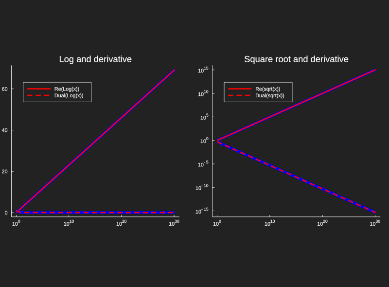
function Log(z::Dual,k=10)    ln2 =  0.6931471805599453094172321214581765680755001343602552541206800094933936219696947156058633269964186875420014810205706857336855202
    b = 0.
    m = z.a
    # use log(ab) = log(a) + log(b) to reduce the magnitute of the logand
    if m > 1
        # find smallest power of 2 larger
        while 2. ^b < m
            b += 1
        end
    elseif m < 1
        # find smallest power of -2 smaller
        while m < 2. ^b
            b -= 1
        end
    end
    # reduce the logand
    z = z / 2. ^b
    L = Dual(0.0,0.0)
    # compute the series with the reduced logand for accuracy
    for i in 0:k
        L += (1/(2*i+1))*((z-Dual(1,0))/(z+Dual(1,0)))^(2*i+1)
    end
    # factor in the logand reduction
    return 2*L + Dual(b*ln2,0.0)
end

function ^(x::Dual,n::AbstractFloat)
    e = 2.7182818284590452353602874713526624977572470936999595749669676277240766303535475945713821785251664274274663919320030599218174135
    y = Log(x,10)
    c = e^(n*y.a)
    return Dual(c,c*(n*y.b))
end
