Implementing Automatic Differentiation 27/11/2020
Differentiation
Calculus is ubiquitous in mathematics applications because it defines
a system for quantifying change. Consider the movement of a ball, the growth
of a portfolio, spread of disease, growth of a bacterial colony, or learning
artificial neural network. All of these problems are intricately linked
to a quantity that changes; to the derivative of a function \(f(x)\).
As humans (or a very advanced AI) we can learn to compute the rate of change
of a function, for example if
$$ f(x) : \mathbb{R}\mapsto\mathbb{R} = x^2 $$
then \(f\)'s rate of change with respect to a change in \(x\) is
$$ \frac{df(x)}{dx} = 2x $$
This comes from the definition of a derivative
$$ f'(x) = \frac{df(x)}{dx} = \lim_{h\rightarrow 0} \frac{f(x+h)-f(x)}{h} $$
i.e the slope of the line \(f(x)\) evaluated between two infinitely close points.
It is possible to define a programming language capable of analytic differentiation
(Mathematica and Wolfram Alpha),
this is not always practical or useful, as such most applications of the derivative
resort to some approximation of the limit definition. Most simply this
can be done by taking an \(h\), say \(h=0.01\), and plugging in the numbers.
This is fine but will lead to errors.
Dual Numbers To the Rescue
It would be nice if for any \(f\) we could know \(f'\) at \(x\) on the fly,
without having to derive it ourselves, approximating it, or asking a computer to chug away and
possibly find the analytic solution itself. This is where dual
numbers come in and reveal "Automatic Differentiation" (AD).
A dual number is a "new" type of number analogous to complex numbers, but now
instead of using \(a+bi\) where \(i=\sqrt{-1}\) we write
$$ a+b\epsilon, \enspace \text{ where } \epsilon^{2}=0, \enspace \text{ for } a,b\in\mathbb{R} $$
This seemingly trivial academic pursuit it incredibly fruitfull. Consider \(f(x)=x^2\), notice
$$f(a+b\epsilon) = a^2 + b^2\cdot(0) + 2ab\epsilon = a^2 + 2ab\epsilon$$
again nothing too crazy, yet, but see that
$$ f(a) = a^2, \text{ and } f'(a) = 2a $$
so if we had taken \(a+\epsilon\) inplace of \(a+b\epsilon\) then we would get
$$f(a+\epsilon) = f(a)+f'(a)\epsilon$$
This is no accident, in fact this result applies to any \(f\) where \(f'\) exists!
$$f(a+b\epsilon) = \sum_{n=0}^{\infty}\frac{f^{(n)}(a)b^n\epsilon^n}{n!} = f(a) + bf'(a)\epsilon + \epsilon^{2}\sum_{n=1}^{\infty}\frac{f^{(n)}(a)b^n\epsilon^n}{n!}$$
So in general evaluating a function of a dual number gives you the value of the function
as it's real part and the exact derivative as it's dual part!
Implementing Dual Numbers
Practically we can make use of these results with a simple object called Dual that
just smashes two Numbers together.
struct Dual{t1<:Number,t2<:Number}
    a::t1
    b::t2
end
Of course the real work is done in defining operators on our objects, in
this case \(+,-,/,*\) for addition, subtraction, division, and multiplication.
import Base.+, Base.*, Base.^, Base.-, Base./

# addition and subtraction are easy
+(x::Dual,y::Dual) = Dual(x.a+y.a,x.b+y.b)
-(x::Dual,y::Dual) = Dual(x.a-y.a,x.b-y.b)

# multiplication (remember that binomial theorem?)
*(x::Dual,y::Dual) = Dual(x.a*y.a,x.a*y.b+x.b*y.a)
*(x::Number,y::Dual) = Dual(x*y.a,x*y.b)
*(y::Dual,x::Number) = *(x::Number,y::Dual)

# division a bit more of a pain
/(x::Dual,y::Dual) = Dual(x.a/y.a,(x.b*y.a-x.a*y.b)/(y.a^2))
/(x::Number,y::Dual) = /(Dual(x,0.),y)
/(y::Dual,x::Number) = /(y,Dual(x,0.))

# positive integer powers
function ^(x::Dual,n::Int)
    y = x
    for i in 1:(n-1)
        y = y*x
    end
    return y
end
At this point the only curve-ball is division, after a bit of algebra
you'd find the expression
$$ \frac{a+b\epsilon}{c+d\epsilon} = \frac{a}{c} + \frac{bc-ad}{c^2}\epsilon $$
which is what we have in the code.
With these definitiions we can make use of AD for functions using integer
powers multiplication division and summation, e.g for powers
julia> [Dual(2^b,1)*Dual(2^b,1) for b in 1:8]
8-element Array{Dual{Int64},1}:
 Dual{Int64}(4, 4)
 Dual{Int64}(16, 8)
 Dual{Int64}(64, 16)
 Dual{Int64}(256, 32)
 Dual{Int64}(1024, 64)
 Dual{Int64}(4096, 128)
 Dual{Int64}(16384, 256)
 Dual{Int64}(65536, 512)
and for \(f(x)=\frac{1}{x}, f'(x)=-\frac{1}{x^2}\)
julia> f = (x) -> 1.0/x
julia> g = (x) -> -(1.0/x^2)
julia> [(1.0/Dual(2^b,1),(f(2^b),g(2^b))) for b in 1:8]
8-element Array{Tuple{Dual{Float64,Float64},Tuple{Float64,Float64}},1}:
 (Dual{Float64,Float64}(0.5, -0.25), (0.5, -0.25))
 (Dual{Float64,Float64}(0.25, -0.0625), (0.25, -0.0625))
 (Dual{Float64,Float64}(0.125, -0.015625), (0.125, -0.015625))
 (Dual{Float64,Float64}(0.0625, -0.00390625), (0.0625, -0.00390625))
 (Dual{Float64,Float64}(0.03125, -0.0009765625), (0.03125, -0.0009765625))
 (Dual{Float64,Float64}(0.015625, -0.000244140625), (0.015625, -0.000244140625))
 (Dual{Float64,Float64}(0.0078125, -6.103515625e-5), (0.0078125, -6.103515625e-5))
 (Dual{Float64,Float64}(0.00390625, -1.52587890625e-5), (0.00390625, -1.52587890625e-5))
Great. But what about other functions like \(\cos\), \(\sin\), \(\exp\), \(\log\)
and real powers (roots etc)? Generally for any function we would make
use of it's Taylor seris (or a faster converging approximation). Let's
look at \(\exp\). The Taylor seris simplifies heavily, i.e
$$e^{a+b\epsilon} = \sum_{n=0}^{\infty}\frac{(a+b\epsilon)^{n}}{n!}=
\sum_{n=0}^{\infty}\frac{1}{n!}\sum_{k=0}^{n}\binom{n}{k}a^{n-k}(b\epsilon)^{k} \\
= \sum_{n=0}^{\infty}\frac{1}{n!}\bigl(a^{n} + na^{n-1}b\epsilon\bigr) = e^{a}(1+b\epsilon)$$
So \(\exp(x)\) can be found exactly with a few muls!
This also means exponentiation to any real power is trivial if we know log...
$$(a+b\epsilon)^{x} = e^{x\log(a+b\epsilon)}$$
$$ \text{Let } \log(a+b\epsilon) = c+d\epsilon$$
$$ (a+b\epsilon)^x = e^{xc}e^{xd\epsilon} = e^{xc}(1+xd\epsilon)$$
Thankfully we can (admittedly approximately) find the natural log just from integer powers, \(*\), and \(/\) !
$$\log(x) = 2\sum_{k=0}^{\infty}\frac{1}{2k+1}\biggl(\frac{x-1}{x+1}\biggr)^{2k+1}$$
This series in particular works nicely for \(x\) about \(1\), which
we can handle by using \(\log(ab) = \log(a)+\log(b)\) to reduce (or increase) the logand
to be about \(1\)
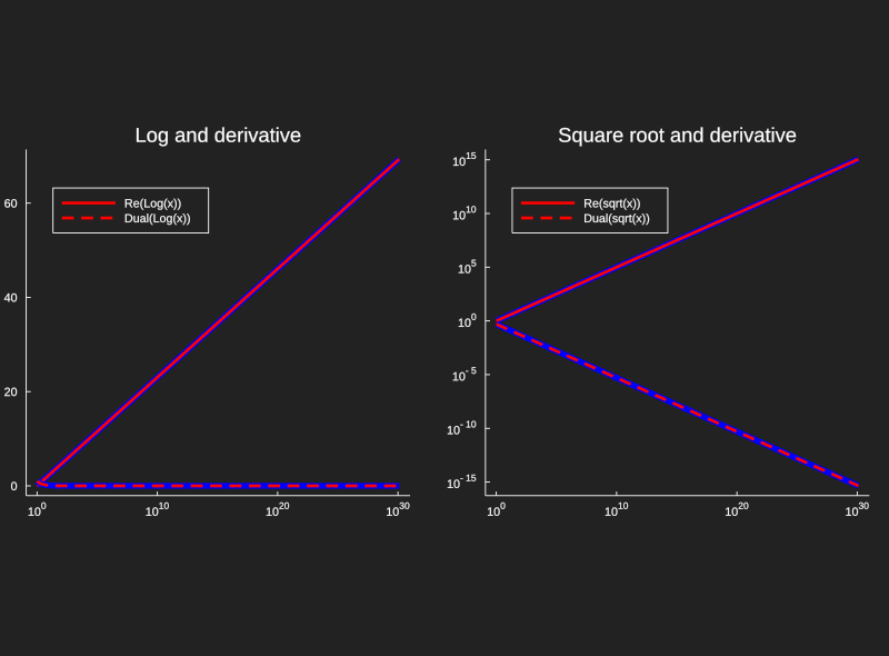
function Log(z::Dual,k=10)
    ln2 =  0.6931471805599453094172321214581765680755001343602552541206800094933936219696947156058633269964186875420014810205706857336855202
    b = 0.
    m = z.a
    # use log(ab) = log(a) + log(b) to reduce the magnitute of the logand
    if m > 1
        # find smallest power of 2 larger
        while 2. ^b < m
            b += 1
        end
    elseif m < 1
        # find smallest power of -2 smaller
        while m < 2. ^b
            b -= 1
        end
    end
    # reduce the logand
    z = z / 2. ^b
    L = Dual(0.0,0.0)
    # compute the series with the reduced logand for accuracy
    for i in 0:k
        L += (1/(2*i+1))*((z-Dual(1,0))/(z+Dual(1,0)))^(2*i+1)
    end
    # factor in the logand reduction
    return 2*L + Dual(b*ln2,0.0)
end

function ^(x::Dual,n::AbstractFloat)
    e = 2.7182818284590452353602874713526624977572470936999595749669676277240766303535475945713821785251664274274663919320030599218174135
    y = Log(x,10)
    c = e^(n*y.a)
    return Dual(c,c*(n*y.b))
end
 This code gives us a quick implementation of dual numbers that we can get some use
out of, but it's far from complete. A real implementation in Julia can be found
as a subpackage of ForwardDiff.jl,
and a great use case for industry is the very elegant machine learning solution Flux.jl
References for Further Reading
[1] - Forward-Mode Automatic Differentiation in Julia,Revels, J. and Lubin, M. and Papamarkou, arXiv:1607.07892 [cs.MS], T. , 2016
 This code gives us a quick implementation of dual numbers that we can get some use
out of, but it's far from complete. A real implementation in Julia can be found
as a subpackage of ForwardDiff.jl,
and a great use case for industry is the very elegant machine learning solution Flux.jl