Link to this blog post as a generated standalone page

Consensus 13/06/2020

Part of this post (the application to flocking) is implemented on my Github

Consensus is "a generally accepted opinion or decision among a group of people" (Cambridge Dictionary). More interestingly the state of consensus around a particular issue can evolve over time, through discussion and debate of ideas.

To think about this mathematically we will first take a leap into graph theory. A group of people can be described as a network, where each person is connected to some (or maybe all) of the others. The most obvious example of this is the social network we construct between friends and family, here "connectedness" just means person $A$ is friends with person $B$.



In the visual representation the people (nodes) are circles and the friendship status (connectivity) between people are represented by lines drawn between them.

Moving back to consensus we can use the network by saying that each person has a current decision $x_i(t)$, where $i$ is an integer representing the individual and $t$ is time. Here we've implied that a persons "decision" is represented as some number, that can also vary as time progresses. The way in which this number varies for each person (the different $i$'s) will be linked to the edges in the network.

If we imagine that $x_2(0)$ is a representation of person $2$'s opinion about a topic at time $0$, it would make sense if the people person $2$ is friends with, $3$ and $5$ from the network, could change person $2$'s opinon i.e change $x_2(0)$. As a first go we might say that a person's opinion changes proportionaly to the difference between their opinion, and the average of the friend's opinions. We can even rigPPht this down for person $2$ $$x_2(1)=\frac{x_3(0)-x_2(0)+x_5(0)-x_2(0)}{2}=\frac{x_5(0)+x_3(0)}{2}-x_2(0)$$ Intuitively this means if person $2$'s opinion is higher (remember "opinions" are numbers here) than $3$ and $5$'s then $2$'s opinion will decrease towards $3$ and $5$'s based upon how different their views are (on average).

Borrowing some more graph theory we can summarise "who knows who" by a $N\cdot N$ grid of numbers, if there are $N$ people, called an "Adjacency Matrix". Think of this as a table with a row and a column for each person, as we read one row $2$ across the columns, when there is a $1$ this tells us person $2$ is friends with the person represented by this column, when there is a $0$ person $2$ is not friends with them.



The image above show a visual representation of this adjacency matrix, here a black square means "not friends" and a yello one means "friends", or as numbers $0$ and $1$. Mathematically we can write this down as $$\mathit{A}=\left[\begin{array}{cccccc}0& 0& 0& 0& 0& 0\\ 0& 0& 1& 0& 1& 0\\ 0& 1& 0& 0& 0& 0\\ 0& 0& 0& 0& 1& 0\\ 0& 1& 0& 1& 0& 1\\ 0& 0& 0& 0& 1& 0\end{array}\right]$$ Where notice that unhelpfully the mathematics convention has it flipped with repspect to the image! Either way we can now say ${\mathit{A}}_{32}=1$, or in plain language the value at the $3$rd row and $2$nd column is $1$.

So how does this relate to our consensus problem? Well we cna begin to genralise how we write down how each person influences the others, e.g for the example from before we can now write $$x_2(1)=\frac{A_{23}}{2}(x_3(0)-x_2(0))+\frac{A_{25}}{2}(x_5(0)-x_2(0))$$ This hasn't changed much yet, but it means we can write the general equation for any $i$! $$x_i(t)=\frac{\sum _{j\ne i}{\mathit{A}}_{ij}(x_j(t-1)-x_i(t-1))}{\sum _{j\ne i}{\mathit{A}}_{ij}}$$ Where the mathematical notation $\sum _i$ means a summation over the index $i$, so $\sum _{i=1}^{5}i=1+2+3+4+5$, and $\ne$ means not equal to, therefore $\sum _{j\ne 2}{\mathit{A}}_{2j}$ means summing over the columns of the grid of numbers ignoring where the column is equal to the row $2$, i.e the number of friends person $2$! Which is $2$

To wrap up, we have a general equation for how each person influences the others opinions in their friendship group, but what is consensus? Looking back at our original definition consensus would mean that everyone shares the same opinion, i.e $$x_1(t)=x_2(t)=x_3(t)=x_4(t)=x_5(t)=x_6(t)$$ And it turns out that we can prove how long it will take before this consensus condition is met, that is when a graph is fully connected, in our example person $1$ is on their own and so won't change their opinion ever under this model!

As a final note, the maths here does not just describe social networks and opinions, we can apply the same reasoning to any process by which multiple "agents" choose a desision and influence the decisions of others, some examples are politics (voter models), collective motion (e.g bird flocks), distributed computation, and swarm robotics.

The pdf below contains the full detail of mathematics, and some applications.

Link to this blog post as a generated standalone page

DNA 16/07/2020

---

What is it?

DNA (Deoxyribonucleic Acid) is the physical mechanism by which many organisms store instructions for their developement and function, and this genetic code is resonsible for traits such as eye colour and many others in humans. Skipping the detailed chemistry, many will be familiar with the idea of DNA as the double helix; two chains of molecules linked together and forming helical twists. The molecules forming DNA in humans go by the names of Adenine (A), Thymine (T), Guanine (G), and Cytosine (C) and are themselves complicated molecular structures.

For our purpose we will take it as given that DNA is formed of these molecules in two chains: one chain which encodes actual information, and a second chain which exists to aid stability. This second chain is formed by two simple rules (in standard DNA), simply if the first chain has an A at a particular position then the second will have a T (and vice versa) but if a G or C is in the first chain the second will have a C or G in the same position respectively. So an example of a valid pair of chains is $$ACACTCAGCGGT$$ $$TGTGAGTCGCCA$$ and an invalid example is $$GCGGTTGATTAA$$ $$CCCCAACGAATT$$

---

The Maths: Number Systems and Bases

Mathematically speaking the interesting part about DNA is that we have exactly four characters to play with. Consider computers, in the computer world all information (including numbers) is represented with just a sequence of $1$s and $0$s; ON and OFF signals in an electrical circuit. The language of computers is Binary. So then what, mathematically speaking, is the language of DNA? Well there are four characters, so it's four-ary more commonly known as Quarternary numbers. What we are dealing with here are different number systems, called bases.

Let's take a step back a second and think about the numbers we are all familiar with, the decimal numbers $0,1,2,3,4,5,6,7,8,9,10,11,\dots$. We call these base-$10$, because there are $10$ digits ($0$ to $9$) that make up how we write down any number, although we of course use a $.$ to represent fractional numbers but this is a notational convenience. So let's throw down a few equations $$0=0\times {10}^0,6=6\times {10}^0,27=2\times {10}^1+7\times {10}^0,172=1\times {10}^2+7\times {10}^1+2\times {10}^0$$ These appear obvious, and they are, but there is a pattern here. Notice we are writing base-$10$ numbers and we see $10$ appearing in every number. Specifically we can write any base-$10$ number as a sum of powers of $10$ each multiplied by just one of the of the $10$ digits $0,1,2,3,4,5,6,7,8,9$. and really our notation $325$ is a shorthand for "3 lots of 100, 2 lots of 10, and 5 lots of 1". Again remarking on this it's obvious, what's the point it's just how it is? The point is that for any base we can generalise this to write numbers in that base, so in Binary , we have to character $0$ and $1$ and instead of powers of $10$ a number will be a sum of powers of $2$ each multiplied by either a $0$ or a $1$ e.g $${101}_2=1\times 2^2+0\times 2^1+1\times 2^0=5=5\times {10}^0=5_{10}$$ where I'm now writing a subscript $x_b$ to say that the number $x$ is to be understood as being written in base $b$. So in maths we like to genralise everything, so we can now write down any (integer for now) number in any base as the sum $$x_b=d_{N-1}{d}_N\cdots d_1{d}_0=d_{N-1}\times b^{N-1}+d_{N-2}\times b^{N-2}+\cdots +d_1\times b^1+d_0\times b^0=\sum _{i=0}^N{d}_i{b}^i$$ where $x_b$ is a number in base $b$ with $N$ digits $d_0,d_1,d_2,\dots d_{N-1}$. For fractional values we can relax the low bound of the sum index $i$ to be -$M$, where $M$ is the number of decimal places, notice this will naturally give negative powers and so fractions.

Armed with this we can return to DNA, we already noticed that DNA has for characters therefore we can think of each character as a digit in a base four number system. Identifying $A=0,C=1,G=2,T=3$ we can write a string of DNA as a number $$ATCGTGC\equiv {0312321}_4={3513}_{10}$$ Since we have represented DNA in base four, we can convert it to any other base. Tricks exist for conversion, and I'm not going to write these down in detail, essentially to go from base $10$ to base $b$ we can use devision and remainder to convert e.g (with all numbers in base $10$) $$143/4=35\text{ remainder }3$$ $$35/4=8\text{ remainder }3$$ $$8/4=2\text{ remainder }0$$ $$2/4=0\text{ remainder }2$$ and (you can check for yourself) $${143}_{10}={2033}_4$$

---

Text to DNA and Back Again

Now that we have learned all of this what can we do with it? Well one fun application is that since computers use base $2$, DNA can be written in base $4$, and we can convert bases we can write DNA as Binary or Binary as DNA. More interestingly since computers often display text, text must be represented as (Binary) numbers somehow, so can we convert text into a DNA sequence? Yes!

Unfortunately there is one slight bump in the road, yes text is written in Binary for computers, but for humans who program computers it is actually more convenient to encode text as base-16 numbers! Of course, we can actually just ignore that for this post since we know how to convert bases (in the future I may even write about base-16, AKA Hexadecimal numbers).

For now though before playing with the code, there is one point to clear up. We can convert from text (Binary/Hex) to base-$4$ easy enough, and we know how base pairs form so the second DNA strand will be automatically taken care of, but how can we decode the information conatining strand? How do we know when when a sequence of DNA should be read as a character? Since there are more than four letters we want to encode, a single letter is going to be formed of multiple base-$4$ digits. DNA also has this problem, it exists to be read, so DNA evolved a solution (which is also studied in the theory of codes like Morse-code) stop sequences. A stop sequence tells us that the characters we have read up to now should be interpreted as a single piece of information (a letter in our case), DNA itself also includes start sequences for extra safety. One DNA stop sequence is $TAG$, which is what we will be using. Let's look at an example, say (arbitrarily) that the sequences $ATAC,GCAT,AC,CTG$ represent the letters "dna!" to encode this as a DNA sequence (with our stop characters so that we can decode it later) we simply write down the sequence. $$\text{"dna!" }\equiv ATACTAGGCATTAGACTAGCTGTAG$$ But this introduces a new problem, what if a letter is represented by $TAGC$ or $GTAG$? Programmatically we can handle this by reading the DNA sequence in fours, we read a set of four DNA characters and convert it to a letter, then we skip the next three characters which should be $TAG$ and read the next four until the end of the sequence. We can even check that the three characters after a letter are $TAG$ to make sure the DNA sequence is not corrupted somehow.

The grand finale then is a program which we can use to re-write any sequence of text as a strand of DNA! As mentioned before I've implemented this in Julia (DNAText.jl [Julia]), and also on this site I've made a Javascript application you can try for yourself!

Link to the this blog post as a generated standalone page

Gaussian Moments 20/08/20

---

Normal Distributions

The Gaussian distribution (or normal distribution) is ubiquitous in mathematics and its applications. Most outside of science will have encountered it as the "Bell curve" when taking or talking about IQ tests and other standardised measurements, or perhaps in an introductory statistics course.

In the wild normal distributions crop up all the time, due to a result known as the central limit theorem. Which states that when we take a sample $\{X_i{\}}_{i=1}^N$ of random numbers with some (finite) mean $\mu$ and (finite) variance ${\sigma }^2$ the variable $Z=\frac{\frac{1}{N}\sum _i{X}_i-\mu }{\sigma /\sqrt{N}}$ will be normally distributed when $N$ is sufficiently large. This is useful for statistical models of real world processes. Since even if data is not "normal" we can "standardise" it, by transforming to $Z(\{X_i\})$, this standardised data can then be put through the various statistical tests statisticians have developed. This was particulary useful before computers, where any sample (sufficiently large!) could be standardised and compared to the same book of "statistical tables".

A great example of a wild normal distribution is the Galton board, shown as a gif below. What we see here are pebbles falling through a set of pegs. On hitting a peg we can assume a pebble has two options, fall left or right with some probability $p$, and given enough pebbles we hope this probability is roughly consistent (despite pebble-pebble collisions). Thankfully it does work, and we end up with a Binomial distribution in the final slots. What's more, given enough pebbles this approximates a normal distribution by the central limit theorem!

The Maths

Let's look at the functional form of a normal distribution. $$p(x)=\frac{1}{\sqrt{2\pi {\sigma }^2}}{e}^{-\frac{(x-\mu {)}^2}{2{\sigma }^2}},-\mathrm{\infty }\le x\le \mathrm{\infty }$$ The exponential gives us a strong concentration of density around the mean $\mu$ which decays of depending on the magnitude of the variance ${\sigma }^2$. High variance means more spread, and a low variance mean a stronger peak and a thinner spread, with the special case of $\sigma \to 0$ being a dirac delta functional picking out the mean.

Shape

These ideas of location and shape are not just applicable to the Gaussian distribution, in fact they form an integral part of how distributions are categorised. Let's remind ourselves what the mean and variance actually are in terms of $p(x)$. If the random variable $X$ is defined by the probability density function $p(x)$, on the range $\mathrm{\Omega }$ the the mean and variance are $$\mathbb{E}[X]={\int }_{x\in \mathrm{\Omega }}xp(x)dx$$ $$\text{Var}[X]={\int }_{x\in \mathrm{\Omega }}(x-\mathbb{E}[X]{)}^{2}p(x)dx$$ For the mean the equation translates as "the sum of all possible values $x$ of $X$ multiplied by their probabilities of occuring", for the variance the equation means "the sum of all square deviations of all possible values of $x$ of $X$ from the mean of $X$ multiplied by their probability of occuring". It's a bit of a mouthfull but essentially it tells us the average distance between realisations of a random variable $X$ from the mean value.

Notice that both these integral functions actually come from the same family $$\{{\int }_{x\in \mathrm{\Omega }}(x-c{)}^{k}p(x)dx:c\in \mathrm{\Omega },k\in \mathbb{N}\}$$ Where $\mathbb{N}=\{1,2,3,\dots \}$. In particular the mean is the element with $k=1$ and $c=0$ and the variance is the element with $k=2$ and $c=\mathbb{E}[X]$. This family is known as the $k$-th moments centered on $c$, higher moments are also useful (but more complicated!) such as $k=3$ which is related to the Skewness of a distribution, and $k=4$ which is related to the peakedness of the distribution (kurtosis). The next figure shows a few of these values off, for the Normal $\mathcal{N}$, Exponential $Exp$ and Binomial $Bin$ distributions.

Fractional Moments

So far so good, but what about the restriction on $k$ that we slipped in? Namely $k\in \mathbb{N}$. Well the "problem" of course is that, when $k=1/2$ say, some distributions like the normal distribution, are defined over negative values. Since $\sqrt{-1}$ is a complex number suddenly some of the moments are not so easy to interpret. Fractional moments may not be quite as intutive as their integer cousins, but nothing is gained without exploring. For the standard normal distribution the fractional moments are defined by the function $z(k):\mathbb{R}\mapsto \mathbb{C}$ $$z(k)=\frac{1}{\sqrt{2\pi }}{\int }_{-\mathrm{\infty }}^{\mathrm{\infty }}{x}^k{e}^{-\frac{x^2}{2}}dx$$ To get an idea of what this thing does, we can approximate this integral numerically. The plots below are valid for steps of $dx=0.01,dk=0.005$ over the range $(-100,100)$. So not quite $(-\mathrm{\infty },\mathrm{\infty })$, but still beautiful!

Link to the this blog post as a generated standalone page

Implementing Automatic Differentiation 27/11/2020

---

Differentiation

Calculus is ubiquitous in mathematics applications because it defines a system for quantifying change. Consider the movement of a ball, the growth of a portfolio, spread of disease, growth of a bacterial colony, or learning artificial neural network. All of these problems are intricately linked to a quantity that changes; to the derivative of a function $f(x)$.

As humans (or a very advanced AI) we can learn to compute the rate of change of a function, for example if $$f(x):\mathbb{R}\mapsto \mathbb{R}=x^2$$ then $f$'s rate of change with respect to a change in $x$ is $$\frac{df(x)}{dx}=2x$$ This comes from the definition of a derivative $$f^{\prime }(x)=\frac{df(x)}{dx}=\underset{h\to 0}{lim}\frac{f(x+h)-f(x)}{h}$$ i.e the slope of the line $f(x)$ evaluated between two infinitely close points. It is possible to define a programming language capable of analytic differentiation (Mathematica and Wolfram Alpha), this is not always practical or useful, as such most applications of the derivative resort to some approximation of the limit definition. Most simply this can be done by taking an $h$, say $h=0.01$, and plugging in the numbers. This is fine but will lead to errors.

Dual Numbers To the Rescue

It would be nice if for any $f$ we could know $f^{\prime }$ at $x$ on the fly, without having to derive it ourselves, approximating it, or asking a computer to chug away and possibly find the analytic solution itself. This is where dual numbers come in and reveal "Automatic Differentiation" (AD).

A dual number is a "new" type of number analogous to complex numbers, but now instead of using $a+bi$ where $i=\sqrt{-1}$ we write $$a+bϵ,\text{ where }{ϵ}^2=0,ϵ\ne 0\text{ for }a,b\in \mathbb{R}$$ This seemingly trivial academic pursuit it incredibly fruitfull. Consider $f(x)=x^2$, notice $$f(a+bϵ)=a^2+b^2\cdot (0)+2abϵ=a^2+2abϵ$$ again nothing too crazy, yet, but see that $$f(a)=a^2,\text{ and }{f}^{\prime }(a)=2a$$ so if we had taken $a+ϵ$ inplace of $a+bϵ$ then we would get $$f(a+ϵ)=f(a)+f^{\prime }(a)ϵ$$ This is no accident, in fact this result applies to any $f$ where $f^{\prime }$ exists! $$f(a+bϵ)=\sum _{n=0}^{\mathrm{\infty }}\frac{f^{(n)}(a)b^n{ϵ}^n}{n!}=f(a)+b{f}^{\prime }(a)ϵ+{ϵ}^2\sum _{n=1}^{\mathrm{\infty }}\frac{f^{(n)}(a)b^n{ϵ}^n}{n!}$$ So in general evaluating a function of a dual number gives you the value of the function as it's real part and the exact derivative as it's dual part!

Implementing Dual Numbers

Practically we can make use of these results with a simple object called Dual that just smashes two Numbers together.

struct Dual{t1<:Number,t2<:Number}
    a::t1
    b::t2
end

Of course the real work is done in defining operators on our objects, in this case $+,-,/,\ast$ for addition, subtraction, division, and multiplication.

import Base.+, Base.*, Base.^, Base.-, Base./

# addition and subtraction are easy
+(x::Dual,y::Dual) = Dual(x.a+y.a,x.b+y.b)
-(x::Dual,y::Dual) = Dual(x.a-y.a,x.b-y.b)

# multiplication (remember that binomial theorem?)
*(x::Dual,y::Dual) = Dual(x.a*y.a,x.a*y.b+x.b*y.a)
*(x::Number,y::Dual) = Dual(x*y.a,x*y.b)
*(y::Dual,x::Number) = *(x::Number,y::Dual)

# division a bit more of a pain
/(x::Dual,y::Dual) = Dual(x.a/y.a,(x.b*y.a-x.a*y.b)/(y.a^2))
/(x::Number,y::Dual) = /(Dual(x,0.),y)
/(y::Dual,x::Number) = /(y,Dual(x,0.))

# positive integer powers
function ^(x::Dual,n::Int)
    y = x
    for i in 1:(n-1)
        y = y*x
    end
    return y
end

At this point the only curve-ball is division, after a bit of algebra you'd find the expression $$\frac{a+bϵ}{c+dϵ}=\frac{a}{c}+\frac{bc-ad}{c^2}ϵ$$ which is what we have in the code. With these definitiions we can make use of AD for functions using integer powers multiplication division and summation, e.g for powers

julia> [Dual(2^b,1)*Dual(2^b,1) for b in 1:8]
8-element Array{Dual{Int64},1}:
 Dual{Int64}(4, 4)
 Dual{Int64}(16, 8)
 Dual{Int64}(64, 16)
 Dual{Int64}(256, 32)
 Dual{Int64}(1024, 64)
 Dual{Int64}(4096, 128)
 Dual{Int64}(16384, 256)
 Dual{Int64}(65536, 512)

and for $f(x)=\frac{1}{x},f^{\prime }(x)=-\frac{1}{x^2}$

julia> f = (x) -> 1.0/x
julia> g = (x) -> -(1.0/x^2)
julia> [(1.0/Dual(2^b,1),(f(2^b),g(2^b))) for b in 1:8]
8-element Array{Tuple{Dual{Float64,Float64},Tuple{Float64,Float64}},1}:
 (Dual{Float64,Float64}(0.5, -0.25), (0.5, -0.25))
 (Dual{Float64,Float64}(0.25, -0.0625), (0.25, -0.0625))
 (Dual{Float64,Float64}(0.125, -0.015625), (0.125, -0.015625))
 (Dual{Float64,Float64}(0.0625, -0.00390625), (0.0625, -0.00390625))
 (Dual{Float64,Float64}(0.03125, -0.0009765625), (0.03125, -0.0009765625))
 (Dual{Float64,Float64}(0.015625, -0.000244140625), (0.015625, -0.000244140625))
 (Dual{Float64,Float64}(0.0078125, -6.103515625e-5), (0.0078125, -6.103515625e-5))
 (Dual{Float64,Float64}(0.00390625, -1.52587890625e-5), (0.00390625, -1.52587890625e-5))

Great. But what about other functions like $\cos$, $\sin$, $\exp$, $\log$ and real powers (roots etc)? Generally for any function we would make use of it's Taylor seris (or a faster converging approximation). Let's look at $\exp$. The Taylor seris simplifies heavily, i.e $$\begin{gathered} e^{a+bϵ}=\sum _{n=0}^{\mathrm{\infty }}\frac{(a+bϵ{)}^n}{n!}=\sum _{n=0}^{\mathrm{\infty }}\frac{1}{n!}\sum _{k=0}^n(\genfrac{}{}{0ex}{}{n}{k})a^{n-k}(bϵ{)}^k \\ =\sum _{n=0}^{\mathrm{\infty }}\frac{1}{n!}(a^n+n{a}^{n-1}bϵ)=e^a(1+bϵ) \end{gathered}$$ So $\exp (x)$ can be found exactly with a few muls! This also means exponentiation to any real power is trivial if we know log... $$(a+bϵ{)}^x=e^{x\log (a+bϵ)}$$ $$\text{Let }\log (a+bϵ)=c+dϵ$$ $$(a+bϵ{)}^x=e^{xc}{e}^{xdϵ}=e^{xc}(1+xdϵ)$$ Thankfully we can (admittedly approximately) find the natural log just from integer powers, $\ast$, and $/$ ! $$\log (x)=2\sum _{k=0}^{\mathrm{\infty }}\frac{1}{2k+1}(\frac{x-1}{x+1}{)}^{2k+1}$$ This series in particular works nicely for $x$ about $1$, which we can handle by using $\log (ab)=\log (a)+\log (b)$ to reduce (or increase) the logand to be about $1$

function Log(z::Dual,k=10)
    ln2 =  0.6931471805599453094172321214581765680755001343602552541206800094933936219696947156058633269964186875420014810205706857336855202
    b = 0.
    m = z.a
    # use log(ab) = log(a) + log(b) to reduce the magnitute of the logand
    if m > 1
        # find smallest power of 2 larger
        while 2. ^b < m
            b += 1
        end
    elseif m < 1
        # find smallest power of -2 smaller
        while m < 2. ^b
            b -= 1
        end
    end
    # reduce the logand
    z = z / 2. ^b
    L = Dual(0.0,0.0)
    # compute the series with the reduced logand for accuracy
    for i in 0:k
        L += (1/(2*i+1))*((z-Dual(1,0))/(z+Dual(1,0)))^(2*i+1)
    end
    # factor in the logand reduction
    return 2*L + Dual(b*ln2,0.0)
end

function ^(x::Dual,n::AbstractFloat)
    e = 2.7182818284590452353602874713526624977572470936999595749669676277240766303535475945713821785251664274274663919320030599218174135
    y = Log(x,10)
    c = e^(n*y.a)
    return Dual(c,c*(n*y.b))
end

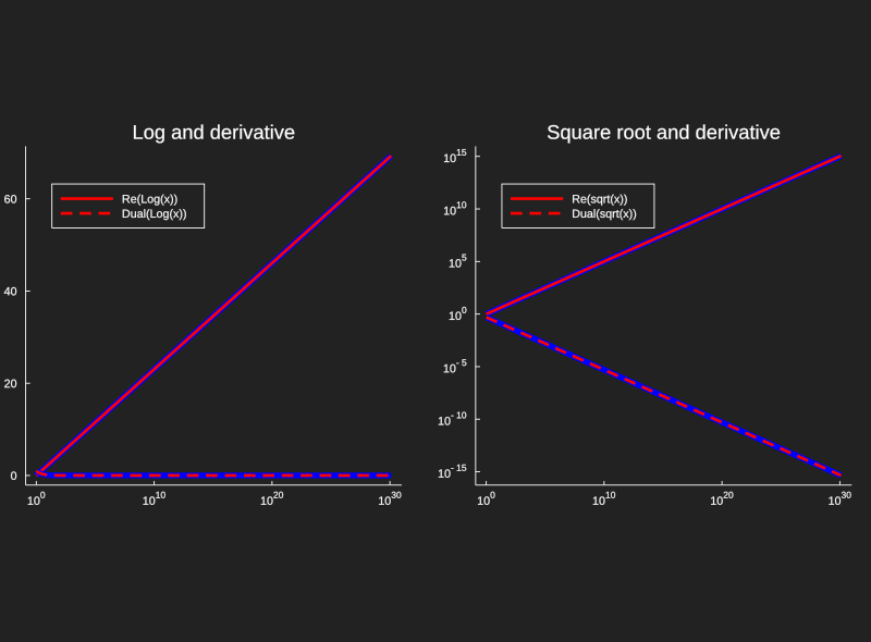This code gives us a quick implementation of dual numbers that we can get some use out of, but it's far from complete. A real implementation in Julia can be found as a subpackage of ForwardDiff.jl, and a great use case for industry is the very elegant machine learning solution Flux.jl

References for Further Reading

[1] - Forward-Mode Automatic Differentiation in Julia,Revels, J. and Lubin, M. and Papamarkou, arXiv:1607.07892 [cs.MS], T. , 2016